Observation: Time-Commodity
Sample period: 1990-2019
Financial Theory: Empirical research has found that found positive historical returns together with low or even slightly negative equity-commodity correlations and positive inflation-commodity correlations. This model may help exploit this arbritrage opportunity. However, the Efficient Market Hypothesis holds that asset prices reflect all available information - eliminating arbitrage opportunities. The predictive data the is being gathered is widely available and commodities are traded continuously at large volumes.

Data Cleaning

Data was cleaned in this file.

Points of Interest

GDP is computed quarterly, so the ‘nearest’ method is used to fill in missing GDP data.
Commodity price and climate data are merged with macroeconomic data to create one DataFrame.
Commodity prices are translated to float types, then used to calculate returns. A sample of this is below.

Unnecessary columns are removed, common timeframes are implimented, and a final DataFrame is created by merging all cleaned data. Cleaned data is exported to a CSV file for reusability.

Commodities_Final['realized_ret_corn'] = (np.log(Commodities_Final['Corn_Future_Price'].shift(-1)) 
                                       - np.log(Commodities_Final['Corn_Future_Price']))
                                       

Regression

The file containing regressions on our data can be found here.

The goal of using regression on our data is to gain an initial understanding of the degree of correlation between the various independent variable in our dataset and the explanatory variables (returns of commodity futures).

These regressions examine the relationship between commodity returns the data described above.

Market Risk Premium Varibale

Computed the monthly returns for the sp500.
Used the .rolling() function to compute a rolling, 60 month period average of the s&p 500 returns.
Calculated estimates for the market risk premium for each observation in our dataset by subtracting a monthly risk free - rate (0.407%) from our s&p 500 returns.
Used a weighted average to ensure positive market risk premiums.
This variable is crucial for the regressions.

With all variables loaded in, the StatsModels library and API are used for regressions. Code and analysis for regressions are below.

Corn Regressions

Model 1: corn1 = sm_ols('realized_ret_corn ~ (market_risk_prem)',data=Commodities_DF).fit()
- Key Statistics:
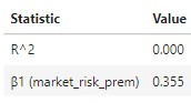
- Interpretation:
  - β1 : A single % increase in the market risk premium is associated with a 0.355% increase in corn future returns, on average.
Model 2: corn2 = sm_ols('realized_ret_corn ~ market_risk_prem + ret_gdp + ret_cpi + UNRATE + sp500_rets', data=Commodities_DF).fit()
- Key Statistics:
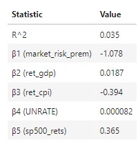
- Interpretation:
  - β1 : A single % increase in the market risk premium is associated with a 1.078% decrease in corn future returns, on average (ceteris paribus).
  - β2: A single % increase in US GDP is associated with with a 0.018% increase in corn future returns, on average (ceteris paribus).
  - β3: A single % increase in US CPI (inflation) is associated with a 0.394% decrease in corn future returns, on average (ceteris paribus).
  - β4: A single % increase in US unemployment rates is associated with a 0.000082% increase in corn future returns, on average (ceteris paribus).
  - β5: A single % increase in SP500 returns is associated with a 0.365% increase in corn future returns, on average (ceteris paribus).
Model 3: sm_ols('realized_ret_corn ~ market_risk_prem + ret_gdp + ret_cpi + UNRATE + sp500_rets + C_PRCP + C_SNOW + C_TMAX + C_TMIN', data=Commodities_DF).fit()
- Key Statistics:
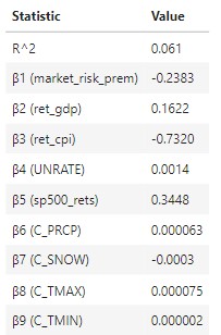
  - Interpretation:
    - β1 : A single % increase in the market risk premium is associated with a -0.2383 decrease in corn future returns, on average (ceteris paribus).
    - β2: A single % increase in US GDP is associated with with a 0.1622% increase in corn future returns, on average (ceteris paribus).
    - β3: A single % increase in US CPI (inflation) is associated with a -0.7320% decrease in corn future returns, on average (ceteris paribus).
    - β4: A single % increase in US unemployment rates is associated with a 0.0014% increase in corn future returns, on average (ceteris paribus).
    - β5: A single % increase in SP500 returns is associated with a 0.3448% increase in corn future returns, on average (ceteris paribus).
    - β6: A single unit increase in precipitation is associated with a 0.000063% increase in corn future returns, on average (ceteris paribus).
    - β7: A single unit increase in snowfall is associated with a -0.0003 increase in corn future returns, on average (ceteris paribus).
    - β8: A single unit increase in max temperatures is associated with a 0.000075% increase in corn future returns, on average (ceteris paribus).
    - β9: A single unit increase in min temperatures is associated with a 0.000002% increase in corn future returns, on average (ceteris paribus).

Soybeans Regressions

Model 1: sm_ols('realized_ret_soybeans ~ (market_risk_prem)',data=Commodities_DF).fit()
- Key Statistics:
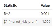
- Interpretation:
  - β1 : A single % increase in the market risk premium is associated with a 1.556% decrease in soybeans future returns, on average.
Model 2: sm_ols('realized_ret_soybeans ~ market_risk_prem + ret_gdp + ret_cpi + UNRATE + sp500_rets', data=Commodities_DF).fit()
- Key Statistics:
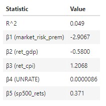
- Interpretation:
  - β1 : A single % increase in the market risk premium is associated with a 2.907% decrease in soybeans future returns, on average (ceteris paribus).
  - β2: A single % increase in US GDP is associated with with a 0.580% decrease in soybeans future returns, on average (ceteris paribus).
  - β3: A single % increase in US CPI (inflation) is associated with a 1.207% decrease in soybeans future returns, on average (ceteris paribus).
  - β4: A single % increase in US unemployment rates is associated with a 0.000009% increase in soybeans future returns, on average (ceteris paribus).
  - β5: A single % increase in SP500 returns is associated with a 0.371% increase in soybeans future returns, on average (ceteris paribus).
Model 3: sm_ols('realized_ret_corn ~ market_risk_prem + ret_gdp + ret_cpi + UNRATE + sp500_rets + C_PRCP + C_SNOW + C_TMAX + C_TMIN', data=Commodities_DF).fit()
- Key Statistics:
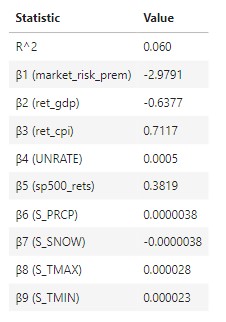
  - Interpretation:
    - β1 : A single % increase in the market risk premium is associated with a 2.979 decrease in soybeans future returns, on average (ceteris paribus).
    - β2: A single % increase in US GDP is associated with with a 0.6377% decrease in soybeans future returns, on average (ceteris paribus).
    - β3: A single % increase in US CPI (inflation) is associated with a 0.7117% increase in soybeans future returns, on average (ceteris paribus).
    - β4: A single % increase in US unemployment rates is associated with a 0.0005% increase in soybeans future returns, on average (ceteris paribus).
    - β5: A single % increase in SP500 returns is associated with a 0.3819% increase in soybeans future returns, on average (ceteris paribus).
    - β6: A single unit increase in precipitation is associated with a 0.0000038% increase in soybeans future returns, on average (ceteris paribus).
    - β7: A single unit increase in snowfall is associated with a 0.0000038 decrease in soybeans future returns, on average (ceteris paribus).
    - β8: A single unit increase in max temperatures is associated with a 0.000028% increase in soybeans future returns, on average (ceteris paribus).
    - β9: A single unit increase in min temperatures is associated with a 0.000023% increase in soybeans future returns, on average (ceteris paribus).

Wheat Regressions

Model 1: sm_ols('realized_ret_wheat ~ (market_risk_prem)',data=Commodities_DF).fit()
- Key Statistics:
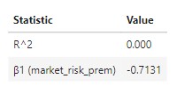
- Interpretation:
  - β1 : A single % increase in the market risk premium is associated with a 0.713% decrease in wheat future returns, on average.
Model 2: sm_ols('realized_ret_wheat ~ market_risk_prem + ret_gdp + ret_cpi + UNRATE + sp500_rets', data=Commodities_DF).fit()
- Key Statistics:
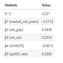
- Interpretation:
  - β1 : A single % increase in the market risk premium is associated with a 3.211% decrease in wheat future returns, on average (ceteris paribus).
  - β2: A single % increase in US GDP is associated with with a 0.344% increase in wheat future returns, on average (ceteris paribus).
  - β3: A single % increase in US CPI (inflation) is associated with a 0.203% increase in wheat future returns, on average (ceteris paribus).
  - β4: A single % increase in US unemployment rates is associated with a 0.0015% decrease in wheat future returns, on average (ceteris paribus).
  - β5: A single % increase in SP500 returns is associated with a 0.358% increase in wheat future returns, on average (ceteris paribus).
Model 3: sm_ols('realized_ret_wheat ~ market_risk_prem + ret_gdp + ret_cpi + UNRATE + sp500_rets + W_PRCP + W_SNOW + W_TMAX + W_TMIN' ,data=Commodities_DF).fit()
- Key Statistics:
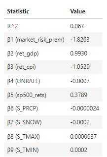
  - Interpretation:
    - β1 : A single % increase in the market risk premium is associated with a 1.8263 decrease in wheat future returns, on average (ceteris paribus).
    - β2: A single % increase in US GDP is associated with with a 0.993% increase in wheat future returns, on average (ceteris paribus).
    - β3: A single % increase in US CPI (inflation) is associated with a 1.0529% decrease in wheat future returns, on average (ceteris paribus).
    - β4: A single % increase in US unemployment rates is associated with a 0.0007% decrease in wheat future returns, on average (ceteris paribus).
    - β5: A single % increase in SP500 returns is associated with a 0.3789% increase in wheat future returns, on average (ceteris paribus).
    - β6: A single unit increase in precipitation is associated with a 0.0000024% decrease in wheat future returns, on average (ceteris paribus).
    - β7: A single unit increase in snowfall is associated with a 0.0002 decrease in wheat future returns, on average (ceteris paribus).
    - β8: A single unit increase in max temperatures is associated with a 0.0000037% increase in wheat future returns, on average (ceteris paribus).
    - β9: A single unit increase in min temperatures is associated with a 0.0002% increase in wheat future returns, on average (ceteris paribus).

Analysis of regressions

Regressions got better as more independent variables as added. Model 3 had the highest R2 among all commodities.
Macroeconomic and climate variables DO help predict variations in futures returns.
Climate coefficients are generally very close to zero, indicating that they are very weakly correlated to returns.
The signs of the coefficients do make sense, as one would expect more precipitation to have a positive impact on crop returns, while the opposite would be the expectation for snowfall.
The coefficient of the market risk premium went from being positive to strongly negative (for corn and soybeans) as other variables were added. This coefficient is essentially an estimate of the financial beta of these futures, so a negative beta is the logical expectation, given that equity and commodity market tend to move in opposite directions.
Most of coefficients observed for all models have a low likelihood to be truly statistically significant, as only a handful of them have a t-score above the threshold value of 1.96.

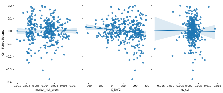
Visualizing Regression Relationships

Visualization 1: Monthly Corn Futures Returns vs Select Independent Variables
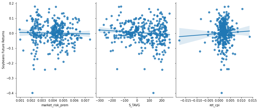
Visualization 2: Monthly Soybeans Futures Returns vs Select Independent Variables
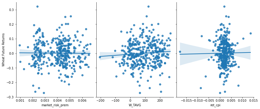
Visualization 3: Monthly Wheat Futures Returns vs Select Independent Variables
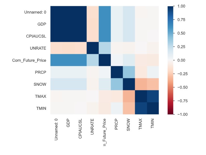
Visualization 4: Heatmap of variables in the corn dataset.

Predictive Modeling

The file containing our predictive machine learning models can be found here.

Step 1: Load Commodity DF, Create Holdout Set
We separated the data to create training and holdout sets. The training set would be used to train the model, whereas the holdout set would be used to test the accuracy of our trained model. Data from years 1990 - 2014 (80%) was used as the training data to create a model for our testing data consisting of years 2015-2019 (20%).

X variables (independent) are separated from the y variable (dependent) for the model. In this case, commodity returns are the dependent variable.

Step 2: EDA on Training Set
EDA was performed on all data, specifically using Pandas Profiling. Few instances of NaN values were found. The data was generally clean. This process was instrimental in understanding the data for accurate modeling.

Step 3: Preprocess Data
To preprocess the data, we created a pipe that would impute numerical NaN variables with their mean, and then used StandardScaler() to scale all of our variables. Within our preproc_pipe, we used the following 8 independent variables within our corn model:

‘ret_gdp’: monthly return of domestic GDP
‘ret_cpi’: monthly return of domestic CPI (Consumer Price Index)
‘UNRATE’: monthly unemployment rate, domestic
‘C_PRCP’: monthly precipitation
‘C_SNOW’: monthly snow
‘C_TMAX’: monthly temperature (max)
‘C_TMIN’: monthly temperature (min)
‘market_risk_prem’: market risk premium (monthly)

Preprocessing was repeated for wheat and soybeans.

Step 4: Create Pipeline
We tried a variety of models to best fit our training set. Models we tried include ridge, lasso, OLS, random forest, Bayesian Ridge, gradient boosting, and elastic net.

The following was the pipeline we used, which resulted in the best fit:

gbr_pipe = Pipeline([
                ('preproc', preproc_pipe),
                ('feature_select', 'passthrough'),
                ('estim', linear_model.BayesianRidge())
                ])

Step 5: Optimizing Hyperparameters and Grid Search

We found that the parameters that highly influence the BayesianRidge() Model were the following:

estim__alpha_1
estim__alpha_2
estim__lambda_1
estim__lambda_2

Because we were predicting future returns, we needed to use a different cross validation (cv) than simply KFold(10). Specifically it was imperative that the splits for the cross validation always had newer data for the holdout set, and older data for the training set, since the entire goal of this project is to test the possibility of using financial theory, macroeconomic, and climatological data to predict future commodity returns. As a result, we set up a type of TimeSeriesSplit cv model. For the calculation of our cv, see below:

groups = X_train.groupby(X_train['DATE'].dt.year).groups
min_periods_in_train = 5
training_expanding_window = True

sorted_groups = [list(value) for (key, value) in sorted(groups.items())]

if training_expanding_window:

    cv = [([i for g in sorted_groups[:y] for i in g],sorted_groups[y]) 
            for y in range(min_periods_in_train , len(sorted_groups))]

else:
    
    cv = [([i for g in sorted_groups[y-min_periods_in_train:y] for i in g],sorted_groups[y]) 
            for y in range(min_periods_in_train, len(sorted_groups))]

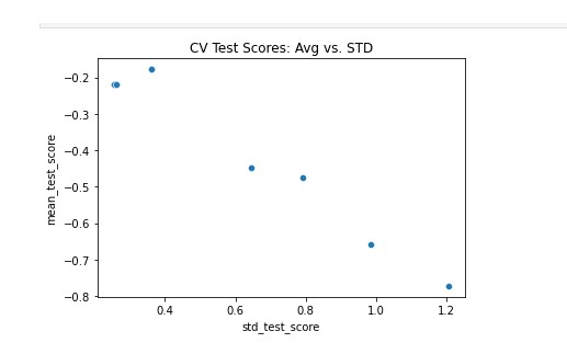
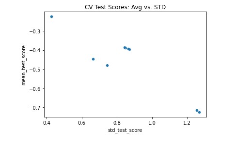
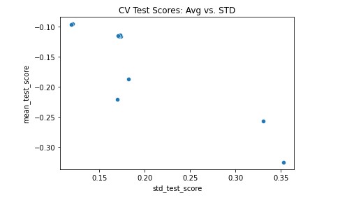
In plotting the candidate models from our grid search, it became clear that our best corn model ended up having a mean_test_score (R^2) value of -0.17827 with a std_test_score of 0.360155. Results were similar for both soybeans and wheat.

While these scores may appear quite underwhelming, we believe that they are optimal for the type of model that we’re building and given that data at our disposal. As previously mentioned, the machine learning model that produced these results was a Bayesian Ridge model. This is another type of a linear model supported by sklearn, that essentially combines the approaches to regularization that Ridge and Lasso models undertake, which is why the model features two alpha and two lambda parameters. The ultimate purpose of those parameters is to limit the likelihood that the beta coefficients associated with our x-variables significantly varied from zero.

Corn
corn_candidates
Soybeans
soybeans_candidates
Wheat
wheat_candidates

Step 6: Test Model on Holdout Set

With an optimal model yielding a negative R^2, we did not expect a good turnout on our holdout set. The following were the respective R^2 values once tested on our holdout set.

1. Corn: 0.00622

2. Soybeans: -0.00307

3. Wheat: 0.00136

With such low R^2 values for all of our commodities, despite trying hundreds of models, we learned that is incredibly difficult to predict future returns simply based on historical information. If anything, this has solidified our expectation of the Efficient Market Hypothesis, which states as such!

Conclusion

Our research determined that the Efficient Market Hypothesis holds for commodity returns. While we were able to explain some of the variation in commodity returns using various financial, macroeconomic, and climate variables (up to 6.7%) in the same time period, we found that these variables do not hold any significant predictive ability when trying to use them to predict future commodity returns. As a result, we are left to conclude that the random walk theory holds for commodity-based assets.

About the Team

Michael Rich is a Financial Engineering major in Lehigh University’s IBE program. He can be reached at mbr223@lehigh.edu.

Alex Outkou is a Finance and Business Information Systems double major at Lehigh University. He can be reached at ado323@lehigh.edu.

Luke Costello is pursuing a degree in Finance at Lehigh University. He can be reached at lrc224@lehigh.edu

Harry Herman is a Finance major at Lehigh University. He can be reached at hsh423@lehigh.edu.

To view the final analysis report associated with this project, click here.
To view the GitHub repo for this website, click here.